SCOT in a Nutshell

SCOT is a novel multipurpose software that incorporates the benefits of a multitude of approaches for the classification of helices, strands, and turns in proteins. To our knowledge, it is the very first method that not only captures a variety of rare and basic secondary structure elements (right- and left-handed α-, 310-, 2.27-, plus right-handed π-helices, PPII helices, and β-sheets) in protein structures, but also their irregularities in a single step, and provides proper output and visualization options.

SCOT combines the benefits of geometry-based and hydrogen bond-based methods by using hydrogen bond and geometric information to gain insights into the structural space of proteins. Its dual character enables robust classifications of secondary structure elements without major influence on the geometric regularity of the assigned secondary structure elements. In consequence, it is perfectly suited to automatically assign secondary structure elements for subsequent helix- and strand-based protein alignments with methods such as LOCK2 [2]. This is especially supported by our elaborate kink detection. All of these benefits are clearly demonstrated by our results. Together with the easy to use visualization of assignments by the means of PyMOL [3] and Chimera [3] scripts, SCOT enables a comprehensive analysis of regular backbone geometries in protein structures.

Key Features

Underlying Methodology

• Dihedral angles
• Hydrogen bonds
• Geometry

Helices

• Right-handed α-, 310-, 2.27-, and π-helices
• Left-handed α-, 310-, 2.27-helices
• Polyproline II helices
• Helix class purity
• Helix kinks

β-sheets

• Sheet assignment
• Strand kinks

Turns

• Normal, reverse, and open turns
• Hydrogen bond energy (normal, reverse) and Cα-distance (open) output

Input

• PDB file [4]

Output

• PDB file [4]
• Secondary structure elements only (in PDB file format)
• PyMOL [4] visualization script
• Chimera [4] visualization script

SCOT is a secondary structure element classification method (SSAM) using hydrogen bonds, geometric properties (Cα–Cα distances), as well as dihedral angles (based on turn clustering).

It supports the classification of helices, β-strands and turns. It reads and writes files in the well-established PDB file format [4].

SCOT requires standard PDB files as input. All options can be set via command line arguments. A list of all supported arguments and a short documentation can be evoked using --help. In addition, trained ESOM files are required for the dihedral angle-based classification of turns.

Our PDB file parsing procedure relies on the information given in the lines with the following prefixes: REMARK 465 (for the support of missing residues), SEQRES (for the support of modified residues), ATOM, HETATM (modified residues), TER, and ENDMDL in NMR structures. We parse the residues according to the ATOM and HETATM lines in the order of their appearance.

SCOT utilizes a hierarchical assignment of protein structural elements starting with the assignment of turns. Since most of the publicly available protein structures in the PDB do not contain information on hydrogen atoms, we use the algorithm by McDonald and Thornton [5] to assign them artificially.

Hydrogen Atom Placement

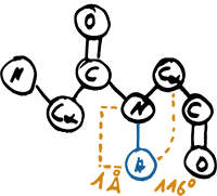
For the determination of the hydrogen-bonded normal and reverse turns, we utilize the DREIDING [6] instead of the established DSSP (Define Secondary Structure of Proteins) [7] hydrogen bonding criterion. For the open turns, we determine the Cα–Cα distance between the first and the last residue of the turn. The detected turns are then clustered according to their dihedral angles.

We use a dataset of more than 3,500 protein structures from the PDB with distinct sequences by the use of the PISCES sequence culling server [8]. The dihedral angles of the classified turns of these proteins are transformed using our Jigsaw-transformation consisting of two functions to address the challenges of a metric distance measure in angular space. The transformed dihedral angles, i.e., two transformed angles for each input angle, are then clustered by emergent self organizing maps (ESOMs) [9], with up to more than 1,000,000 neurons for a single class, resulting in a variety of distinct turn clusters of similar backbone conformations.

Turn Categories, Hydrogen Bonds, and Cα–Cα Distances

Jigsaw Transformation

The next layer of the hierarchical assignment of secondary structure elements is dedicated to the classification of sheets and strands. We have developed three algorithms to assign sheets and strands. The final one determines the hydrogen bond contacts for all residues of an input protein structure. Using these contacts, we build a strand graph consisting of sequence regions of consecutive parallel or anti- parallel hydrogen bonding patterns. The edges are labeled with the hydrogen bonds they represent connecting different strands. Thus, each strand, and its length in particular, is implicitly defined by the hydrogen bond information stored at the labels of its vertex’ incident edges.

We then determine a merge blocking fingerprint based on specific turns which are usually located between succeeding strands within the same sheet. Using this fingerprint, we merge consecutive strands whose gap is not indicated as blocked by this fingerprint. Each connected component of the graph represents a sheet, each of which consisting of at least two strands.

To cope with the circularity of β-barrels and to guarantee a deterministic assignment of sheets and strands, we use a priority queue to extract the sheet and strand information out of the graph. During this step, we also determine kinks based on the Cα–Cα distances in segments of length 4 in a strand. If this distance falls below a pre-defined threshold, a kink is defined.

The additional information about kinks is added to the REMARK section of the output PDB file to be conform to the PDB file format.

Strand Scheme

The final layer of the hierarchical assignment of secondary structure elements deals with the classification of helices. We have developed five different algorithms for this purpose. The final one classifies right-handed (α, 310, π), left-handed (α, 310), and ribbon (polyproline II, 2.27) helices. Each of these three groups is processed separately. In each such group and for each class of a helix (e.g., α), the turn overlaps of all sequence positions of the corresponding turn (i.e., normal of length 5 and class 1) are determined. Plus, we also determine the turn overlaps of the corresponding open turns for all helix classes within one group. These are used for the extension of our helices.

Based on the class-specific and extension overlaps, we define three layered helices consisting of a core, a hull, and an extension. Each such helix is created whenever we detect a segment of succeeding helix-specific turn overlaps of a minimum number of overlaps and segment length. This is the core of the helix. The hull is defined as all neighboring residues with an overlap of at least 1. The extension is defined according to the core but based on the extension overlaps.

We then split and block these helices whenever the Cα–Cα distance of a sequence segment of length 4 within a helix exceeds a predefined threshold. After that, we merge consecutive and overlapping helices and determine their classification based on the sequence coverage and turn overlaps for each involved helix class. The dominant class is taken as the final helix class. We also determine a helix class Purity based on these overlaps to reflect the dominance of a helix’ class.

We finally assign kinks within cores and hulls based on minima in the corresponding turn overlaps. We also assign classes to kinks to reflect the different geometrical regions a helix can consist of (e.g., 15 for a kink between an α (1) and 310 (5) core).

The information about kinks and class Purity are added to the REMARK section.

Core Helix Layers

Core Helix Splitting

For each PDB input file, we write a PDB output file containing the SCOT secondary structure element assignment and optional PyMOL [9] or Chimera [9] visualization scripts on request using the command line option --write-pymol or --write-chimera, respectively.

The PDB output file contains all lines from the PDB input file except for the HELIX, SHEET, TURN, REMARK 650, REMARK 700, and REMARK 750 lines. The HELIX and SHEET lines are given in PDB format. The REMARK lines contain information about kinks for helices and strands, helix class purities, and a format description for the TURN lines.

Example PyMOL Script Visualization

• Linux CentOS
  Executable + ESOM files, approx. 262 MB

• 2020-07-24
• Added Chimera [9] output script option
• Bugfixes

Preparation

1. Download the latest version of SCOT from the download section.
2. Extract the archive using the command
   tar -xzvf scot+esoms.tar.gz
3. If neccessary apply execution rights
   chmod u+x scot

Usage

• Call the following command to view the complete usage
  ./scot --help
• Call ./scot 1gos.pdb 1 to classify (single thread) the secondary structure elements for the PDB [9] file 1gos.pdb and add them to this file. Existing secondary structure element information in this file is overwritten.
• Call ./scot 1gos.pdb 1gos_scot.pdb 1 to classify (single thread) the secondary structure elements for the PDB file 1gos.pdb and write a new file with name 1gos_scot.pdb.
• Call ./scot input/ output/ 5 to classify in parallel (5 threads) the secondary structure elements for all *.pdb files in the input directory and write PDB files containing the classified secondary structure elements to the output directory.
• Use the option --write-pymol to write a PyMOL [9] visualization script for each input PDB file.
• Use the option --write-chimera to write a Chimera [9] visualization script for each input PDB file.